1. PINN简介

   PINN是一种利用神经网络求解偏微分方程的方法，其计算流程图如下图所示，这里以偏微分方程(1)为例。
$$\begin{array}{r}\frac{\partial u}{\partial t}+u\frac{\partial u}{\partial x}=v\frac{{\partial }^{2}u}{\partial x^2}\end{array}$$
神经网络输入位置x,y,z和时间t的值，预测偏微分方程解u在这个时空条件下的数值解。

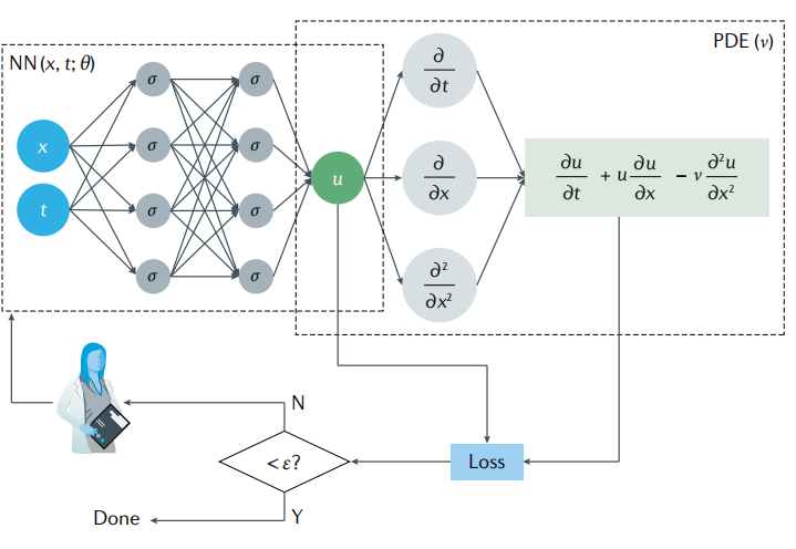
   上图中可以看出，PINN的损失函数包含两部分内容，一部分是来源于训练数据误差，另一部分来源于偏微分方程误差，可以记作(2)式。
$$\begin{array}{r}l=w_{data}{l}_{data}+w_{PDE}{l}_{PDE}\end{array}$$
其中
$$\begin{array}{r}\begin{array}{rl}{l}_{data}& =\frac{1}{N_{data}}\sum _{i=1}^{N_{data}}(u(x_i,t_i)-u_i{)}^2\\ l_{PDE}& =\frac{1}{N_{data}}\sum _{j=1}^{N_{PDE}}{\left(\frac{\partial u}{\partial t}+u\frac{\partial u}{\partial x}-v\frac{{\partial }^{2}u}{\partial x^2}\right)}^2{|}_{(x_j,t_j)}\end{array}\end{array}$$

2. 偏微分方程实例

   考虑偏微分方程如下：
$$\begin{array}{r}\begin{array}{r}\frac{{\partial }^{2}u}{\partial x^2}-\frac{{\partial }^{4}u}{\partial y^4}=(2-x^2)e^{-y}\end{array}\end{array}$$
考虑以下边界条件，
$$\begin{array}{r}\begin{array}{rl}{u}_{yy}(x,0)& =x^2\\ u_{yy}(x,1)& =\frac{x^2}{e}\\ u(x,0)& =x^2\\ u(x,1)& =\frac{x^2}{e}\\ u(0,y)& =0\\ u(1,y)& =e^{-y}\end{array}\end{array}$$
以上偏微分方程真解为$u(x,y)=x^2{e}^{-y}$,在区域$[0,1]\times [0,1]$上随机采样配置点和数据点，其中配置点用来构造PDE损失函数$l_1,l_2,\cdots ,l_7$，数据点用来构造数据损失函数$l_8$.
l1=1N1∑(xi,yi)∈Ω(u^xx(xi,yi;θ)−u^yyyy(xi,yi;θ)−(2−xi2)e−yi)2l2=1N2∑(xi,yi)∈[0,1]×{0}(u^yy(xi,yi;θ)−xi2)2l3=1N3∑(xi,yi)∈[0,1]×{1}(u^yy(xi,yi;θ)−xi2e)2l4=1N4∑(xi,yi)∈[0,1]×{0}(u^(xi,yi;θ)−xi2)2l5=1N5∑(xi,yi)∈[0,1]×{1}(u^(xi,yi;θ)−xi2e)2l6=1N6∑(xi,yi)∈{0}×[0,1](u^(xi,yi;θ)−0)2l7=1N7∑(xi,yi)∈{1}×[0,1](u^(xi,yi;θ)−e−yi)2l8=1N8∑i=1N8(u^(xi,yi;θ)−ui)2\begin{align} \begin{aligned} \mathcal{l}_1 &= \frac{1}{N_1}\sum_{(x_i,y_i)\in\Omega} (\hat{u}_{xx}(x_i,y_i;\theta) - \hat{u}_{yyyy}(x_i,y_i;\theta) - (2-x_i^2)e^{-y_i})^2 \\ \mathcal{l}_2 &= \frac{1}{N_2}\sum_{(x_i,y_i)\in[0,1]\times\{0\}} (\hat{u}_{yy}(x_i,y_i;\theta) - x_i^2)^2 \\ \mathcal{l}_3 &= \frac{1}{N_3}\sum_{(x_i,y_i)\in[0,1]\times\{1\}} (\hat{u}_{yy}(x_i,y_i;\theta) - \frac{x_i^2}{e})^2 \\ \mathcal{l}_4 &= \frac{1}{N_4}\sum_{(x_i,y_i)\in[0,1]\times\{0\}} (\hat{u}(x_i,y_i;\theta) - x_i^2)^2 \\ \mathcal{l}_5 &= \frac{1}{N_5}\sum_{(x_i,y_i)\in[0,1]\times\{1\}} (\hat{u}(x_i,y_i;\theta) - \frac{x_i^2}{e})^2 \\ \mathcal{l}_6 &= \frac{1}{N_6}\sum_{(x_i,y_i)\in\{0\}\times [0,1]}(\hat{u}(x_i,y_i;\theta) - 0)^2 \\ \mathcal{l}_7 &= \frac{1}{N_7}\sum_{(x_i,y_i)\in\{1\}\times [0,1]}(\hat{u}(x_i,y_i;\theta) - e^{-y_i})^2 \\ \mathcal{l}_8 &= \frac{1}{N_{8}}\sum_{i=1}^{N_{8}} (\hat{u}(x_i,y_i;\theta)-u_i)^2 \end{aligned} \end{align} l1​l2​l3​l4​l5​l6​l7​l8​​=N1​1​(xi​,yi​)∈Ω∑​(u^xx​(xi​,yi​;θ)−u^yyyy​(xi​,yi​;θ)−(2−xi2​)e−yi​)2=N2​1​(xi​,yi​)∈[0,1]×{0}∑​(u^yy​(xi​,yi​;θ)−xi2​)2=N3​1​(xi​,yi​)∈[0,1]×{1}∑​(u^yy​(xi​,yi​;θ)−exi2​​)2=N4​1​(xi​,yi​)∈[0,1]×{0}∑​(u^(xi​,yi​;θ)−xi2​)2=N5​1​(xi​,yi​)∈[0,1]×{1}∑​(u^(xi​,yi​;θ)−exi2​​)2=N6​1​(xi​,yi​)∈{0}×[0,1]∑​(u^(xi​,yi​;θ)−0)2=N7​1​(xi​,yi​)∈{1}×[0,1]∑​(u^(xi​,yi​;θ)−e−yi​)2=N8​1​i=1∑N8​​(u^(xi​,yi​;θ)−ui​)2​​​

3. 基于pytorch实现代码

"""
A scratch for PINN solving the following PDE
u_xx-u_yyyy=(2-x^2)*exp(-y)
Author: suntao
Date: 2023/2/26
"""
import torch
import matplotlib.pyplot as plt
from mpl_toolkits.mplot3d import Axes3Depochs = 10000    # 训练代数
h = 100    # 画图网格密度
N = 1000    # 内点配置点数
N1 = 100    # 边界点配置点数
N2 = 1000    # PDE数据点def setup_seed(seed):torch.manual_seed(seed)torch.cuda.manual_seed_all(seed)torch.backends.cudnn.deterministic = True# 设置随机数种子
setup_seed(888888)# Domain and Sampling
def interior(n=N):# 内点x = torch.rand(n, 1)y = torch.rand(n, 1)cond = (2 - x ** 2) * torch.exp(-y)return x.requires_grad_(True), y.requires_grad_(True), conddef down_yy(n=N1):# 边界 u_yy(x,0)=x^2x = torch.rand(n, 1)y = torch.zeros_like(x)cond = x ** 2return x.requires_grad_(True), y.requires_grad_(True), conddef up_yy(n=N1):# 边界 u_yy(x,1)=x^2/ex = torch.rand(n, 1)y = torch.ones_like(x)cond = x ** 2 / torch.ereturn x.requires_grad_(True), y.requires_grad_(True), conddef down(n=N1):# 边界 u(x,0)=x^2x = torch.rand(n, 1)y = torch.zeros_like(x)cond = x ** 2return x.requires_grad_(True), y.requires_grad_(True), conddef up(n=N1):# 边界 u(x,1)=x^2/ex = torch.rand(n, 1)y = torch.ones_like(x)cond = x ** 2 / torch.ereturn x.requires_grad_(True), y.requires_grad_(True), conddef left(n=N1):# 边界 u(0,y)=0y = torch.rand(n, 1)x = torch.zeros_like(y)cond = torch.zeros_like(x)return x.requires_grad_(True), y.requires_grad_(True), conddef right(n=N1):# 边界 u(1,y)=e^(-y)y = torch.rand(n, 1)x = torch.ones_like(y)cond = torch.exp(-y)return x.requires_grad_(True), y.requires_grad_(True), conddef data_interior(n=N2):# 内点x = torch.rand(n, 1)y = torch.rand(n, 1)cond = (x ** 2) * torch.exp(-y)return x.requires_grad_(True), y.requires_grad_(True), cond# Neural Network
class MLP(torch.nn.Module):def __init__(self):super(MLP, self).__init__()self.net = torch.nn.Sequential(torch.nn.Linear(2, 32),torch.nn.Tanh(),torch.nn.Linear(32, 32),torch.nn.Tanh(),torch.nn.Linear(32, 32),torch.nn.Tanh(),torch.nn.Linear(32, 32),torch.nn.Tanh(),torch.nn.Linear(32, 1))def forward(self, x):return self.net(x)# Loss
loss = torch.nn.MSELoss()def gradients(u, x, order=1):if order == 1:return torch.autograd.grad(u, x, grad_outputs=torch.ones_like(u),create_graph=True,only_inputs=True, )[0]else:return gradients(gradients(u, x), x, order=order - 1)# 以下7个损失是PDE损失
def l_interior(u):# 损失函数L1x, y, cond = interior()uxy = u(torch.cat([x, y], dim=1))return loss(gradients(uxy, x, 2) - gradients(uxy, y, 4), cond)def l_down_yy(u):# 损失函数L2x, y, cond = down_yy()uxy = u(torch.cat([x, y], dim=1))return loss(gradients(uxy, y, 2), cond)def l_up_yy(u):# 损失函数L3x, y, cond = up_yy()uxy = u(torch.cat([x, y], dim=1))return loss(gradients(uxy, y, 2), cond)def l_down(u):# 损失函数L4x, y, cond = down()uxy = u(torch.cat([x, y], dim=1))return loss(uxy, cond)def l_up(u):# 损失函数L5x, y, cond = up()uxy = u(torch.cat([x, y], dim=1))return loss(uxy, cond)def l_left(u):# 损失函数L6x, y, cond = left()uxy = u(torch.cat([x, y], dim=1))return loss(uxy, cond)def l_right(u):# 损失函数L7x, y, cond = right()uxy = u(torch.cat([x, y], dim=1))return loss(uxy, cond)# 构造数据损失
def l_data(u):# 损失函数L8x, y, cond = data_interior()uxy = u(torch.cat([x, y], dim=1))return loss(uxy, cond)# Trainingu = MLP()
opt = torch.optim.Adam(params=u.parameters())for i in range(epochs):opt.zero_grad()l = l_interior(u) \+ l_up_yy(u) \+ l_down_yy(u) \+ l_up(u) \+ l_down(u) \+ l_left(u) \+ l_right(u) \+ l_data(u)l.backward()opt.step()if i % 100 == 0:print(i)# Inference
xc = torch.linspace(0, 1, h)
xm, ym = torch.meshgrid(xc, xc)
xx = xm.reshape(-1, 1)
yy = ym.reshape(-1, 1)
xy = torch.cat([xx, yy], dim=1)
u_pred = u(xy)
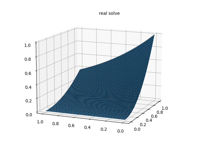
u_real = xx * xx * torch.exp(-yy)
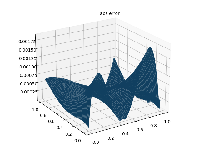
u_error = torch.abs(u_pred-u_real)
u_pred_fig = u_pred.reshape(h,h)
u_real_fig = u_real.reshape(h,h)
u_error_fig = u_error.reshape(h,h)
print("Max abs error is: ", float(torch.max(torch.abs(u_pred - xx * xx * torch.exp(-yy)))))
# 仅有PDE损失    Max abs error:  0.004852950572967529
# 带有数据点损失  Max abs error:  0.0018916130065917969# 作PINN数值解图
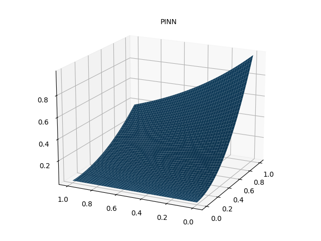
fig = plt.figure()
ax = Axes3D(fig)
ax.plot_surface(xm.detach().numpy(), ym.detach().numpy(), u_pred_fig.detach().numpy())
ax.text2D(0.5, 0.9, "PINN", transform=ax.transAxes)
plt.show()
fig.savefig("PINN solve.png")# 作真解图
fig = plt.figure()
ax = Axes3D(fig)
ax.plot_surface(xm.detach().numpy(), ym.detach().numpy(), u_real_fig.detach().numpy())
ax.text2D(0.5, 0.9, "real solve", transform=ax.transAxes)
plt.show()
fig.savefig("real solve.png")# 误差图
fig = plt.figure()
ax = Axes3D(fig)
ax.plot_surface(xm.detach().numpy(), ym.detach().numpy(), u_error_fig.detach().numpy())
ax.text2D(0.5, 0.9, "abs error", transform=ax.transAxes)
plt.show()
fig.savefig("abs error.png")

4. 数值解

参考资料

[1]. Physics-informed machine learning
[2]. 知乎-PaperWeekly